
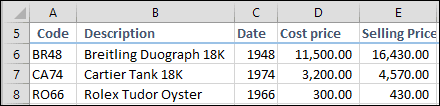


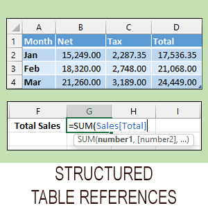

VLOOKUP inexact match
VLOOKUP lesson with sample file that will teach you everything there is to know when creating a VLOOKUP inexact match Excel function.

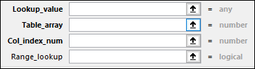
Excel XLOOKUP function (part two)
This is the second of a two-part series of XLOOKUP lessons. If you haven’t already done so I recommend that you begin with part one
Excel XLOOKUP function (part one)
The new Excel XLOOKUP function was introduced in the July 2020 Excel 365 semi-annual update. It isn’t available in older versions (Excel 2019 and earlier).

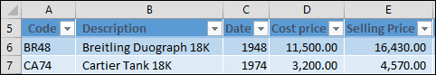
Using VLOOKUP, if Column 1 is blank, get value from Column 2
This article shows how to create an Excel VLOOKUP formula that extracts data from a different column if the first column it searches is blank.
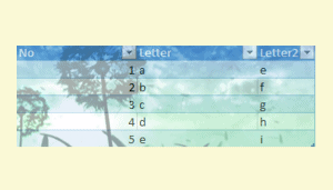
Adding images to tables
This article explains how to insert pictures into Excel workbooks and Excel’s current image features, including cell backgrounds.
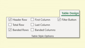
Table Tools, Design Tools Group
This article explains the Table Tools > Design tab on the Excel Ribbon, how to access it and how to reset the Ribbon if the tab has been disabled.