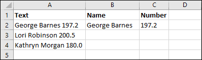
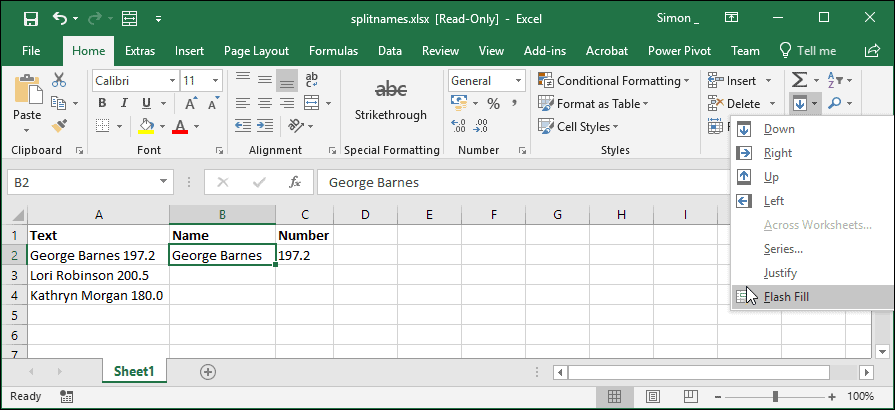
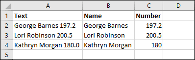


This article describes three different ways of splitting delimited data in Excel, including Flash Fill, Text to Columns and formulas.

This article explains several different ways to carry out an AutoFill using the keyboard in Excel and explains Flash Fill and the Repeat command.
Sometimes you need to know whether a cell contains specific, or any text. This article shows how to do this using the SEARCH, ISNUMBER and FIND functions.


12 Responses
Based on the above advice, it cannot separate text and numbers when numbers are in front of the text, e.g. 12345abcde. Any further advice?
Hi Alex,
All of the above solutions should work with the numbers in front of the text.
For the formula-based approach the difference would be that you would need to search for the last number rather than the first. You could do this by using the MAX function instead of the MIN function.
Once you have the location of the last number you should be able to use the LEFT function to extract all of the numbers.
ACTUALLY THIS IS NOT WORKING FOR ME.
If you can be more specific about what you are trying to do and how it is not working I should be able to offer some advice.
After copying the formula for finding the first numeral, edit the double quote marks in the copy, replacing each of them with your keyboard’s double quote key.
This is a common problem on websites: the articles are written with word processing software which will replace the keyboard typed double quotes with slicker ones (in Word this is called using smart quotes) meant for publishing. And if that does not happen, or is correctly fixed afterward, any processing when loading to the webiste may do it also.
I also have a situation where I need to separate numbers and text in the same cell, where the numbers are in front. I tried using the MAX function and it’s not working for me. What formula could I use to create the result below?
Before: 00868#09ALVARADO
After: 00868#09 ALAVARADO <—There's a space between "9" and "A"
If the two codes have a consistent length you should be able to do this easily using Flash Fill or by using Text To Columns, as mentioned above. If you need a formula-based solution and the codes are always the same length you should also be able to do this easily using the LEFT and RIGHT functions. It’s only in cases where the codes could have a variable length that you will need a formula that searches for the position of the last number or first letter of the code.
The MAX solution will only work correctly if all of the numbers 0-9 can be found in the target, so it might not actually be the best approach in a situation like this. Formulas do exist that can reliably extract the last number from a value without any foreknowledge of what numbers might be present, but they are much more complex.
A simpler solution in this case would be to find the first letter instead of the last number. Assuming the value is in cell A2, you could do that using:
=MIN(FIND({“A”,”B”,”C”,”D”,”E”,”F”,”G”,”H”,”I”,”J”,”K”,”L”,”M”,”N”,”O”,”P”,”Q”,”R”,”S”,”T”,”U”,”V”,”W”,”X”,”Y”,”Z”},A2&”ABCDEFGHIJKLMNOPQRSTUVWXYZ”))-1
This works in exactly the same way as the formula above, but it runs the FIND function 26 times (once for each letter of the alphabet) and returns the lowest result. You can then extract the values on each side using the LEFT, RIGHT and LEN functions.
To get the part before the A you would use:
=LEFT(A2,MIN(FIND({“A”,”B”,”C”,”D”,”E”,”F”,”G”,”H”,”I”,”J”,”K”,”L”,”M”,”N”,”O”,”P”,”Q”,”R”,”S”,”T”,”U”,”V”,”W”,”X”,”Y”,”Z”},A2&”ABCDEFGHIJKLMNOPQRSTUVWXYZ”))-1)
To get the part after the A you would use:
=RIGHT(A2,LEN(A2)-(MIN(FIND({“A”,”B”,”C”,”D”,”E”,”F”,”G”,”H”,”I”,”J”,”K”,”L”,”M”,”N”,”O”,”P”,”Q”,”R”,”S”,”T”,”U”,”V”,”W”,”X”,”Y”,”Z”},A2&”ABCDEFGHIJKLMNOPQRSTUVWXYZ”)))-1)
Now that you have extracted both parts of the value, you could join them back together with a space between them using the & operator, for example:
=B2&” “&C2
Could you please help to find highest value and lowest value from this
please paste the below data in one cell (Ex. A1) and need to find highest value
Cell: A1
a)63Ra b)64Ra c)65Ra d)62Ra e)61Ra f)63Ra g)60Ra h)62Ra
Hi Adaikkala,
I would recommend first breaking each of the items into separate cells, either using Flash Fill or the Text to Columns feature. You can see how to use Flash Fill above, and Text to Columns is covered in this article.
Both skills are covered in depth in our courses.
After the values have been placed in separate cells you should be able to use the skills shown above to extract the numbers and could then use the MAX and MIN functions to determine the highest and lowest.
Thank you very much
=MIN(FIND({0,1,2,3,4,5,6,7,8,9},A2&”0123456789″))
does nothing for me
i tried replacing ” and ; etc even typed it by hand new and it does not work.
the line always just says
=MIN(FIND({0,1,2,3,4,5,6,7,8,9},A2&”0123456789″))
instead of showing the result.
Any thoughts how to fix this?
I’ve just tested this and it worked perfectly for me. With the text “George Barnes 197.2″ in cell A2, the formula: =MIN(FIND({0,1,2,3,4,5,6,7,8,9},A2&”0123456789”)) returned 15 as expected. If you copy and paste from the web page you’ll have to manually re-enter the double quotation marks (web page quotes are different to Excel quotes) but you’ve said that you’ve done that.
My best guess is that it is an Excel version issue. There have been a huge number of Excel versions and some have bugs that others don’t have, some also have functions that others don’t have. All I can report is that it worked perfectly using Excel 365 version 2103 Build 13901.20462 which was the latest version of Excel at time of writing. Having said that, I’d also expect it to work on all other versions of Excel but your experience suggests otherwise!