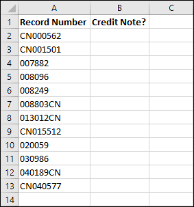
Sometimes you need to search for a specific piece of text within a cell. One example I had to deal with in my professional career was a situation where a workbook combined invoice and credit note data from two different systems. In one system, credit notes had the code CN before the invoice number, but the other placed the CN after the invoice number. I needed to create a formula that could identify which of the records were credit notes.
If you’re already experienced with Excel, you might immediately think of the LEFT, RIGHT and IF functions. Those would offer a solution, but you would need some quite complex formulas. The SEARCH function offers a much easier solution.
If you are interested in the LEFT, RIGHT and IF functions, they are covered in depth in our Expert Skills course.
The SEARCH function
Excel’s SEARCH function searches a cell for a piece of text. It searches the entire cell, so there’s no need to carefully extract the part you need using LEFT, RIGHT and MID functions.
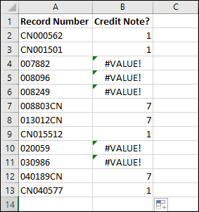
You can search for the text ‘CN’ using the following formula:
=SEARCH(“CN”,A2)
…but that’s only part of the puzzle.
As you can see, the SEARCH function searches for ‘CN’ and returns a number that indicates its position in the cell. You can see that cells A2 and A3 have the text ‘CN’ at position 1 – right at the beginning of the cell. Cells A7 and A8 have it at position 7 – at the end of the cell. If the text isn’t found at all, a #VALUE! error is returned.
Once again there are multiple ways that you could address this, such as the IFERROR function (covered in our Expert Skills course), but I’m going to use the ISNUMBER function.
The ISNUMBER function
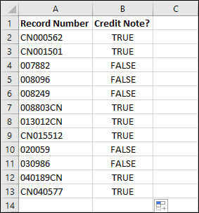
ISNUMER is quite self-explanatory: it returns TRUE if its target contains a number and FALSE if it does not. Combining it with the previous formula gives you this:
=ISNUMBER(SEARCH(“CN”,A2))
This is the result I was looking for. I can now see which of the records were credit notes and I could use this to sort them, filter them, or carry out calculations using functions like SUMIF and COUNTIF.
Before finishing this article, I’d also like to mention the similar FIND function.
The FIND function
FIND works in almost exactly the same way as SEARCH. The only difference is that FIND is case sensitive.
SEARCH is not case sensitive, so any of the following formulas would have had the same result shown above:
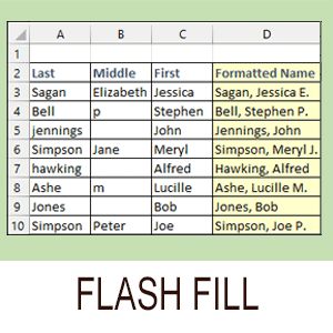
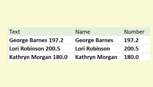
This article shows three different ways of separating text and numbers in Excel. You’ll see how to do this using Flash Fill, Text to Columns and formulas.