Publishers of the world’s most comprehensive and up-to-date Excel tutorials

Excel tutorials

The only Excel books you will ever need

The only constantly updated Excel 365 titles more…
Thoroughly covers Power Pivot and Power Query more…
Covers business intelligence and OLAP features more…
Simple, easy, understandable, 2-page lessons more…
Available as both printed books and e-Books more…
Used by schools, colleges and universities more…
Available for 365, 2021, 2019, 2016 and Mac versions more…

How to hide #N/A errors in Excel

February 12, 2022
2 Comments

What does the #N/A error code mean?

#N/A means “Not Available”. Excel formulas usually return this in situations where a requested value could not be found for some reason.

One of the most common causes of the #N/A error code is the VLOOKUP function. If a VLOOKUP function can’t find a matching value it will return #N/A.

If you’re unfamiliar with Excel formulas and functions you could benefit greatly from our completely free Basic Skills E-book.
All of Excel’s error codes are explained in depth in our Expert Skills Books and E-books.

Hiding #N/A codes

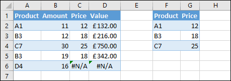
Here is an example:

Column C is using VLOOKUP to return prices from the table in columns F and G. In cell C6 the VLOOKUP function was unable to find a matching product so it returned a #N/A error.

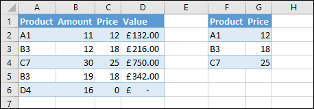
In many cases this is what you would want to happen; if a price is missing it could be a genuine error that needs to be corrected. In some cases you might want to suppress the #N/A error. To do that, you’d use the IFERROR function.

IFERROR allows you to specify what should be returned if an error occurs. To replace any missing prices with zero, you could use this formula:

=IFERROR(VLOOKUP(A6,$F$2:$G$4,2,FALSE),0)

Surrounding the VLOOKUP formula with IFERROR lets you choose what will happen if an error is returned. In this case you’ve specified 0 when an error occurs, but you could make it display “Price Missing” with this formula:

=IFERROR(VLOOKUP(A6,$F$2:$G$4,2,FALSE),”Price Missing”)

IFERROR and VLOOKUP are explained in depth in our Expert Skills Books and E-books.