
Calculated fields allow you to create pivot table fields that carry out calculations. A common example might be multiplying a number by a percentage to calculate taxes.
Our Expert Skills Books and E-books explains calculated fields in depth, but this article focuses on modifying and deleting calculated fields that already exist.
This article uses one of the sample files from our Expert Skills course as an example. If you’d like to follow along you can download a copy:
Modifying a pivot table calculated field
The Insert Calculated Field dialog can be a little confusing to work with. To open it, first click the pivot table, then click:
PivotTable Tools > Analyze > Fields, Items & Sets > Calculated Field…
The Insert Calculated Field dialog appears.
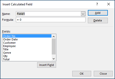
When it first appears, the dialog is ready to insert a new calculated field called Field1. It’s not immediately obvious whether there are any existing calculated fields or how to access them.
If you click the drop-down arrow next to Field1 you will see a list of all of the existing calculated fields, allowing you to select them.
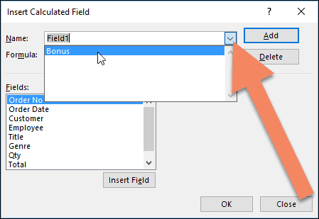
There’s only one existing calculated field in the example workbook, named Bonus.
After selecting the Bonus calculated field you can see that it is currently calculating 3% of the Total field. You’ll also notice that the Add button changes to say Modify.
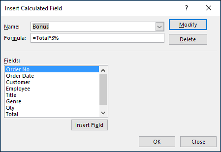
You can now change the formula that is used by the calculated field and click Modify to save your changes or click Delete to delete the calculated field.
You’ll find much more about pivot tables and calculated fields in our Expert Skills Books and E-books, including a complete explanation of the new OLAP pivot tables.


2 Responses
Kindly advise how did you manage to have the Source Name (Cost per Unit) the same as the Custom Name (Cost per Unit) for the pivot table created from the Data worksheet on file Film Sales-2 ( session 8: Exercise – page 369) of Session Eight: Pivot Tables
There’s a trick to this – Excel won’t allow you to name a pivot table column exactly the same thing as one of the data fields the pivot table is based on, but adding an extra space to the end of the name allows you to create a column that looks exactly the same even though it’s technically different.
In the Film Sales-2 sample file, the pivot table field name is “Cost per Unit”, so the column name used is “Cost per Unit ” (notice the extra space).