Excel Challenge #1: Conditional Formatting
Level: Essential Skills, Estimated Completion Time: Under 5 minutes
Sample File
To save you time typing in the data you can download this sample file that has the starting-point for the challenge:
PDF Version
This challenge is also available as a printable PDF file.
If you'd rather watch a video...
Table of Contents
Challenge Overview
Challenge 1: Download the sample file and open it in Excel
Challenge 2: Add an average row
Challenge 3: Improve the appearance of the worksheet
Challenge 4: Add a visualization to show the budget for each film
Challenge 5: Shade each Title cell according to the Wordwide Gross
Challenge 6: Extend the shading in column F across rows A:E
Solution
Challenge Overview
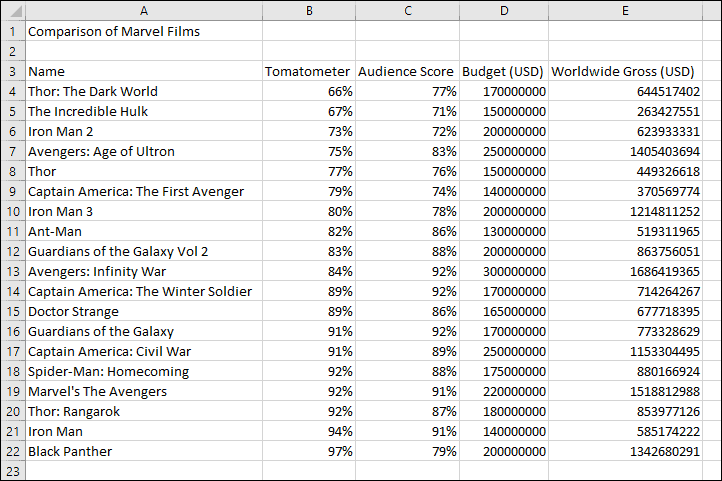
In this challenge you’ll begin with a very basic worksheet that has not been formatted in any way:
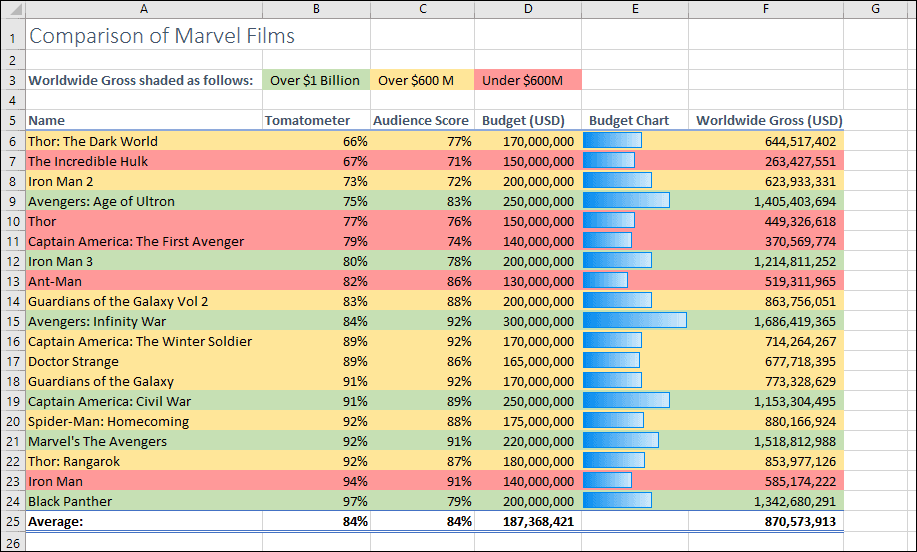
You’ll transform this worksheet into the one shown below that uses many of Excel’s advanced conditional formatting features:
Estimated time to complete this challenge: 4 minutes, 12 seconds
The solution video shows this task being completed in the estimated time shown above.
It is interesting to compare the time a trained Excel user (trained to Essential Skills level only) can complete a simple task when compared to an untrained user. An untrained user could spend many hours figuring out how to complete this task (if they were able to complete it at all) and would probably attempt it in an unnecessarily complex way.
Challenge 1: Download the sample file and open it in Excel
To save you time typing in the data you can download this sample file that has the starting point for the challenge.
The Tomatometer shows the percentage of professional film reviews that are positive while the Audience Score shows the approval rating from members of the general public.
The films are sorted in Tomatometer ascending order. You can see that Thor: The Dark World had the lowest number of professional positive reviews while Black Panther had the highest.
You’ll probably agree that this isn’t a very impressive worksheet. It has all of the information, but it isn’t particularly presentable or easy to read. If an employee created this spreadsheet for you, you might send them on an Excel training course.
Challenge 2: Add an average row
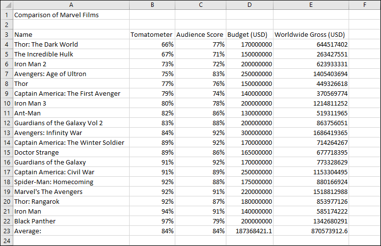
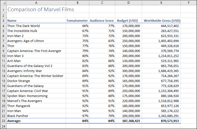
Add averages to row 23 so that the worksheet looks like this:
Tasks
- Add the text Average: to cell A23
- Add formulas to cells B23, C23, D23 and E23 to show the average of all values displayed in the column above.
Estimated time: 17 seconds
There is a way to add average formulas to cells B23:E23 with just three clicks of the mouse.
The solution video shows this task being completed in the estimated time shown above.
Challenge 3: Improve the appearance of the worksheet
Format the worksheet so that it looks the same as the worksheet shown below:
Tasks
- Apply the Title style to cell A1
- Apply the Heading 3 style to cells A3:E3
- Apply the Total style to cells B23:E23
- Display whole numbers in columns D and E (no decimal places) with comma separators.
Hints
If you’re not familiar with Cell Styles you might think that you need to manually apply borders and change font sizes and colors. The correct approach is to use Excel’s Cell Styles feature.
Estimated time: 29 seconds
The solution video shows this task being completed in the estimated time shown above.
Challenge 4: Add a visualization to show the budget for each film
For this challenge you need to make your worksheet look the same as the one shown below. The blue bars must automatically adjust if any of the values in column D change:
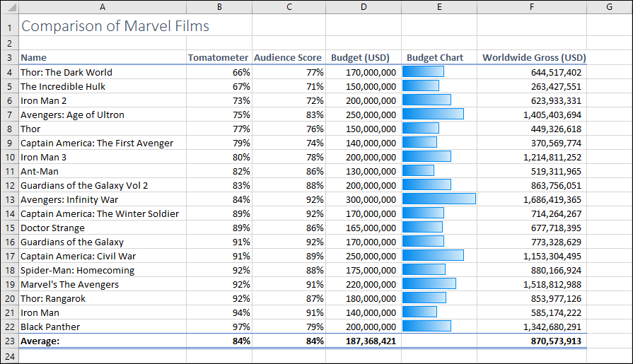
Before the visualization was added it would have taken a few moments for you to tell which of the Marvel films had the highest budget.
The visualization elegantly conveys that Avengers: Infinity War was Marvel’s most expensive film with a budget of twice that for The Incredible Hulk.
Visualizations really make data come alive.
Tasks
- Add a column to the right of the Budget (USD) column.
- Type the column heading: Budget Chart at the top of the new column.
- Add a visualization to cells E4:E22 to visually convey the values shown in cells D4:D22.
Hint
Don’t try to use Sparklines to create the bar chart. The correct approach is to use a visualization.
Estimated time: 33 seconds
The solution video shows this task being completed in the estimated time shown above.
Challenge 5: Shade the Worldwide Gross values to visually identify the best performers
At the end of this challenge your worksheet needs to look like the one shown below:
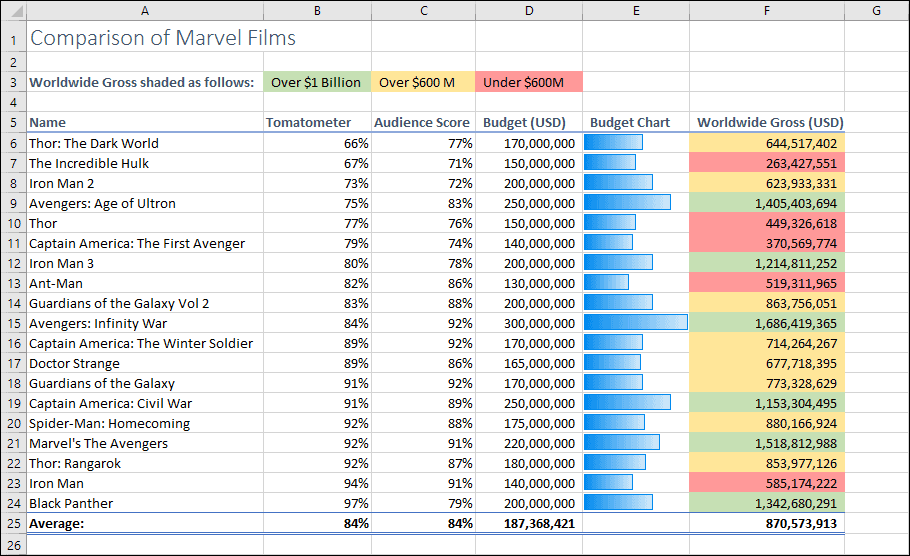
The data now yields some interesting insights at a glance.
- You can instantly identify the six most successful (and five most unsuccessful) films.
- You can see that the critics opinion doesn’t seem to influence the popularity of each film (though there is a strong correlation between the budget spent and the film’s success).
Tasks
- Add a key to the top of the worksheet to indicate what the shading signifies.
- In column F, automatically shade the background color of values that exceed one billion dollars to Green
- In column F, automatically shade the background color of values that are 600 million dollars or less to Red.
Estimated time: 2 minutes, 26 seconds
The solution video shows this task being completed in the estimated time shown above.
Challenge 6: Extend the shading in column F across rows A:E
The shading works well but the worksheet would be more readable if the Wordwide Gross indication color extended across all columns.
Edit the worksheet so that it looks like this:
Hints
If you used mixed cell references in the previous step, you’ll be able to complete this challenge very quickly.
Estimated time: 18 seconds
The solution video shows this task being completed in the estimated time shown above.
Challenge Solution Video Tutorial
Attempt the challenge before watching the solution video
If you have difficulties completing the challenge (or if you want to use our challenges as a learning resource in themselves) we’ve create a professional narrated 26-minute challenge solution video tutorial that fully explains each step needed to complete this challenge. You should only watch the solution video if you have difficulty completing the challenge.
If you do need to work through the challenge solution video tutorial try the challenge again afterwards and keep trying until you can complete it without referring to the video.